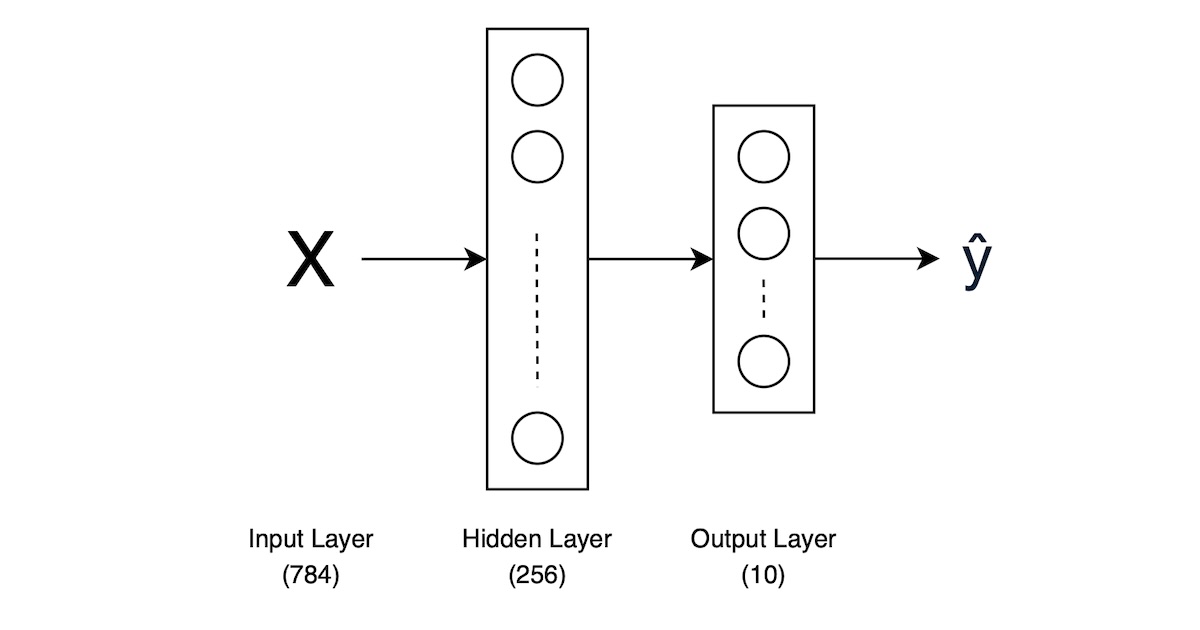
In this post, we will try to implement Multilayer Perceptrons (MLP) from scratch using Pytorch. For illustration purposes, we will use the simplest MLP architecture with only one hidden layer as an example and use FashionMNIST dataset for training and evaluation. This will help us understand the underlying mechanics of MLP and how it can be applied to a multi-class classification task.
Implementation
1. Importing libraries
1
2
3
4
| import torch
import torchvision
from torchvision import transforms
from torch.utils import data
|
2. Initializing parameters
Let’s create a function to initialize the model parameters (weights and bias) that we will optimize during training. As we are using one hidden layer architecture, we need to initialize weights and biases for both the hidden layer and the output layer.
1
2
3
4
5
6
7
8
9
10
11
12
13
14
15
| def init_params(num_inputs: int, num_outputs: int, num_hiddens: int) -> tuple[torch.Tensor, torch.Tensor, torch.Tensor, torch.Tensor]:
"""
Initialize the parameters for the one hidden layer MLP model.
Args:
num_inputs (int): Number of input features.
num_outputs (int): Number of output classes.
num_hiddens (int): Number of hidden units.
Returns:
tuple[torch.Tensor, torch.Tensor, torch.Tensor, torch.Tensor]: Initialized weight matrices and bias vectors.
"""
W1 = torch.normal(0, 0.01, size=(num_inputs, num_hiddens), requires_grad=True)
b1 = torch.zeros(num_hiddens, requires_grad=True)
W2 = torch.normal(0, 0.01, size=(num_hiddens, num_outputs), requires_grad=True)
b2 = torch.zeros(num_outputs, requires_grad=True)
return W1, b1, W2, b2
|
3. Defining the model
The biggest difference between normal linear models and MLPs is the use of activation functions. In this case, we will use the ReLU (Rectified Linear Unit) activation function for the hidden layer.
1
2
3
4
5
6
7
8
9
10
| def relu(X: torch.Tensor) -> torch.Tensor:
"""
Apply the ReLU activation function element-wise.
Args:
X (torch.Tensor): Input tensor.
Returns:
torch.Tensor: Output tensor with ReLU applied.
"""
A = torch.zeros_like(X)
return torch.max(A, X)
|
1
2
3
4
5
6
7
8
9
10
11
12
13
14
15
16
| def mlp(X: torch.Tensor, W1: torch.Tensor, b1: torch.Tensor, W2: torch.Tensor, b2: torch.Tensor) -> torch.Tensor:
"""
Define the forward pass of the one hidden layer MLP.
Args:
X (torch.Tensor): Input tensor with shape (num_samples, num_inputs).
W1 (torch.Tensor): Weights for the first layer with shape (num_inputs, num_hiddens).
b1 (torch.Tensor): Biases for the first layer with shape (num_hiddens,).
W2 (torch.Tensor): Weights for the second layer with shape (num_hiddens, num_outputs).
b2 (torch.Tensor): Biases for the second layer with shape (num_outputs,).
Returns:
torch.Tensor: Output tensor after passing through the MLP with shape (num_samples, num_outputs).
"""
num_inputs = W1.shape[0]
H1 = relu(X.reshape(-1, num_inputs) @ W1 + b1)
H2 = H1 @ W2 + b2
return H2
|
4. Defining the loss function
Create a loss function to measure the difference between predicted and true values. As we know, this is a multi-class classification problem, we’ll use Cross-Entropy Loss as our loss function. And softmax will be applied to the output layer before computing the loss.
1
2
3
4
5
6
7
8
9
10
11
| def softmax(X: torch.Tensor) -> torch.Tensor:
"""
Compute the softmax for each row of the input tensor.
Args:
X: Input tensor of shape (num_samples, num_classes)
Returns:
Output tensor of the same shape as X, containing the softmax probabilities.
"""
X_exp = torch.exp(X)
partition = X_exp.sum(1, keepdim=True)
return X_exp / partition
|
1
2
3
4
5
6
7
8
9
10
| def cross_entropy_loss(y_hat: torch.Tensor, y: torch.Tensor) -> torch.Tensor:
"""
Compute the cross-entropy loss.
Args:
y_hat: Predicted probabilities of shape (num_samples, num_classes)
y: True labels of shape (num_samples,)
Returns:
Scalar tensor representing the cross-entropy loss.
"""
return -torch.mean(torch.log(y_hat[range(len(y_hat)), y]))
|
5. Defining the optimizer
We create a function to update (optimize) parameters using gradient descent.
1
2
3
4
5
6
7
8
9
10
11
12
13
14
15
16
17
18
19
| def updater(W1: torch.Tensor, b1: torch.Tensor, W2: torch.Tensor, b2: torch.Tensor, lr: float) -> None:
"""
Update model parameters using gradient descent.
Args:
W1 (torch.Tensor): Weight tensor for the first layer.
b1 (torch.Tensor): Bias tensor for the first layer.
W2 (torch.Tensor): Weight tensor for the second layer.
b2 (torch.Tensor): Bias tensor for the second layer.
lr (float): Learning rate.
"""
with torch.no_grad():
W1 -= lr * W1.grad
b1 -= lr * b1.grad
W2 -= lr * W2.grad
b2 -= lr * b2.grad
W1.grad.zero_() # Reset gradients
b1.grad.zero_() # Reset gradients
W2.grad.zero_() # Reset gradients
b2.grad.zero_() # Reset gradients
|
6. Creating mini-batch stochastic gradient descent (SGD) iterator
We will use stochastic gradient descent (SGD) for optimization. So we need to create a data iterator that yields mini-batches of data. Here we use Fashion MNIST dataset as an example.
1
2
3
4
5
6
7
8
9
10
11
12
13
14
| def load_data_fashion_mnist(batch_size: int) -> tuple[data.DataLoader, data.DataLoader]:
"""
Load the Fashion MNIST dataset.
Args:
batch_size (int): The number of samples per batch.
Returns:
tuple[data.DataLoader, data.DataLoader]: The training and test data loaders.
"""
trans = transforms.ToTensor()
mnist_train = torchvision.datasets.FashionMNIST(root="./data", train=True, transform=trans, download=True)
mnist_test = torchvision.datasets.FashionMNIST(root="./data", train=False, transform=trans, download=True)
train_iter = data.DataLoader(mnist_train, batch_size=batch_size, shuffle=True)
test_iter = data.DataLoader(mnist_test, batch_size=batch_size, shuffle=False)
return train_iter, test_iter
|
7. Evaluating the accuracy
We create accuracy function to compute the total number of correct predictions and evaluate_accuracy function to evaluate the accuracy of the model with specific parameters on the given data.
1
2
3
4
5
6
7
8
9
10
11
| def accuracy(y_hat: torch.Tensor, y: torch.Tensor) -> float:
"""
Compute the total number of correct predictions.
Args:
y_hat: Predicted probabilities of shape (num_samples, num_classes)
y: True labels of shape (num_samples,)
Returns:
Scalar representing the number of correct predictions.
"""
y_pred = y_hat.argmax(dim=1) # (num_samples,)
return float((y_pred == y).sum())
|
1
2
3
4
5
6
7
8
9
10
11
12
13
14
15
16
17
18
19
| def evaluate_accuracy(data_iter: data.DataLoader, W1: torch.Tensor, b1: torch.Tensor, W2: torch.Tensor, b2: torch.Tensor) -> float:
"""
Evaluate the accuracy of the model on the given data.
Args:
data_iter (data.DataLoader): DataLoader for the dataset.
W1 (torch.Tensor): Weight tensor for the first layer.
b1 (torch.Tensor): Bias tensor for the first layer.
W2 (torch.Tensor): Weight tensor for the second layer.
b2 (torch.Tensor): Bias tensor for the second layer.
Returns:
float: Accuracy of the model on the dataset.
"""
acc_sum, n = 0.0, 0
for X, y in data_iter:
y_hat = mlp(X, W1, b1, W2, b2)
y_hat = softmax(y_hat)
acc_sum += accuracy(y_hat, y)
n += len(y)
return acc_sum / n
|
8. Creating the training function
Since we already defined the model, loss function, and optimizer, we can create the training function to train the model.
1
2
3
4
5
6
7
8
9
10
11
12
13
14
15
16
17
18
19
20
21
22
23
24
25
26
27
28
29
30
31
32
33
34
| def train(
train_iter: data.dataloader.DataLoader, # Training data
test_iter: data.dataloader.DataLoader, # Test data
W1: torch.Tensor, b1: torch.Tensor, # Hidden layer parameters
W2: torch.Tensor, b2: torch.Tensor, # Output layer parameters
num_epochs: int, lr: float # Hyperparameters
) -> None:
"""
Train the multi-layer perceptron (MLP) model.
Args:
train_iter: DataLoader for the training dataset.
test_iter: DataLoader for the test dataset.
W1: Weight tensor for the hidden layer
b1: Bias tensor for the hidden layer
W2: Weight tensor for the output layer
b2: Bias tensor for the output layer
num_epochs: Number of training epochs
lr: Learning rate
"""
for epoch in range(num_epochs):
for X, y in train_iter:
# Forward pass
y_hat = mlp(X, W1, b1, W2, b2)
y_hat = softmax(y_hat)
l = cross_entropy_loss(y_hat, y)
# Backward pass
l.backward()
updater(W1, b1, W2, b2, lr)
# Evaluate on test set
eval_acc = evaluate_accuracy(test_iter, W1, b1, W2, b2)
print(f'Epoch {epoch + 1}, Loss: {l.item():.4f}, Test Accuracy: {eval_acc:.4f}')
|
Test Implementation
Training the model
Now we can train our MLP model using the Fashion MNIST dataset. We’ll iterate through the data in mini-batches, compute predictions, calculate loss, and update the parameters using SGD.
1
2
3
4
5
6
7
8
9
10
11
12
13
14
15
16
17
18
19
20
21
22
23
24
| num_inputs, num_outputs = 28 * 28, 10 # Number of input features and output classes
num_hiddens = 256 # Number of hidden units
num_epochs = 10 # Number of epochs
batch_size = 256 # Number of samples per batch
lr = 0.1 # Learning rate
W1, b1, W2, b2 = init_params(num_inputs, num_outputs, num_hiddens) # Parameters
# Load the data
train_iter, test_iter = load_data_fashion_mnist(batch_size)
# Train the model
train(train_iter, test_iter, W1, b1, W2, b2, num_epochs, lr)
# Epoch 1, Loss: 0.6413, Test Accuracy: 0.7668
# Epoch 2, Loss: 0.5204, Test Accuracy: 0.7882
# Epoch 3, Loss: 0.4691, Test Accuracy: 0.8054
# Epoch 4, Loss: 0.5508, Test Accuracy: 0.8247
# Epoch 5, Loss: 0.3962, Test Accuracy: 0.8022
# Epoch 6, Loss: 0.3901, Test Accuracy: 0.8392
# Epoch 7, Loss: 0.5033, Test Accuracy: 0.8022
# Epoch 8, Loss: 0.4763, Test Accuracy: 0.8257
# Epoch 9, Loss: 0.3368, Test Accuracy: 0.8480
# Epoch 10, Loss: 0.4321, Test Accuracy: 0.8348
|
As the parameters (w, b) were initialized randomly, the loss and accuracy may vary between different runs.
Summary
In this implementation, we have built a multi-layer perceptron (MLP) model (one hidden layer) from scratch using PyTorch. We defined the model, loss function, and optimization algorithm, and trained the model with the Fashion MNIST dataset using mini-batch stochastic gradient descent. The training process involved iterating over the data, computing predictions, calculating loss, and updating the model parameters. After training for a few epochs, we observed a significant reduction in loss, indicating that the model was learning to fit the data.
References